Reveal R code
datatable(roster, rownames=FALSE, options=list(pageLength=5, dom='ltip'))Our DOC captures 10 Evidence Based Recidivism Reduction (EBRR) programs listed by the Federal Bureau of Prisons and the individuals involved:
Your DOC Research Department tracks clients served and staff involved in running and supporting these programs.
Let’s take a look at this EBRR program data. The name of our data is roster. Trying to gather anything from raw data row by row can be painful. We need to explore and synthesize what variables/columns we have, and get a quick summary of what they all look like. We know that GDOC has 10 programs. How can we find out more?
datatable(roster, rownames=FALSE, options=list(pageLength=5, dom='ltip'))#what's in our data
print(dfSummary(roster, varnumbers = FALSE, valid.col = FALSE),
method = "render", footnote = NA)
#capture number of columns for printing in text
numcol <- ncol(roster)| Variable | Stats / Values | Freqs (% of Valid) | Graph | Missing | |||||||||||||||||||||||||||||||||||||||||||||||||||||||
|---|---|---|---|---|---|---|---|---|---|---|---|---|---|---|---|---|---|---|---|---|---|---|---|---|---|---|---|---|---|---|---|---|---|---|---|---|---|---|---|---|---|---|---|---|---|---|---|---|---|---|---|---|---|---|---|---|---|---|---|
| client_names [character] |
|
|
 |
0 (0.0%) | |||||||||||||||||||||||||||||||||||||||||||||||||||||||
| age [numeric] |
|
18 distinct values |  |
0 (0.0%) | |||||||||||||||||||||||||||||||||||||||||||||||||||||||
| dt [Date] |
|
47 distinct values |  |
0 (0.0%) | |||||||||||||||||||||||||||||||||||||||||||||||||||||||
| programs [character] |
|
|
 |
0 (0.0%) | |||||||||||||||||||||||||||||||||||||||||||||||||||||||
| ret [numeric] |
|
|
 |
0 (0.0%) |
From what the summary above shows us, it appears we have 5 variables in the roster dataset. What further exploring, cleaning, and manipulation is required for us to successfully produce results for Director Summers?
What other pieces of information might be relevant to what we need to know about the data? Since it appears to be person-level data from our data exploration summary, let’s check to make sure that there aren’t any duplicate observations.
#are there any duplicates?
roster[duplicated(roster) | duplicated(roster, fromLast=TRUE),]

#how many duplicates?
dupct <- length(unique(
  roster[duplicated(roster) | duplicated(roster, fromLast=TRUE),]
  ))
It’s a really good thing we checked! From the table above it appears we have 5 duplicate observations/rows in our data. Let’s remove them and keep exploring!
#deduplicate across all columns
roster.nodup <- roster[!duplicated(roster), ]


#check for dups again
roster.nodup[duplicated(roster.nodup) | duplicated(roster.nodup, fromLast=TRUE),]
Alright! No more duplicates! What else could require cleaning that we haven’t thought of?
We need to take a closer look at our other variables that may help us report out what the GDOC director needs. Let’s start with our programs, dt, and ret.
#count total number of programs
define_keywords(title.freq = "PROGRAMS values")
print(freq(roster.nodup$programs, report.nas = FALSE, cumul = FALSE, display.type = FALSE),
      method = "render", footnote = NA, Variable = "")

#count number of programs
prgnum <- n_distinct(roster.nodup$programs)| Freq | % | |
|---|---|---|
| am | 7 | 14.00 |
| bcs | 3 | 6.00 |
| bgs | 1 | 2.00 |
| brave | 6 | 12.00 |
| brv | 2 | 4.00 |
| challenge | 6 | 12.00 |
| dbt | 2 | 4.00 |
| fbt | 1 | 2.00 |
| mhsd | 3 | 6.00 |
| rdap | 3 | 6.00 |
| rdp | 1 | 2.00 |
| resolve | 3 | 6.00 |
| sotrt | 3 | 6.00 |
| stages | 9 | 18.00 |
| Total | 50 | 100.00 |
#check out weird date values
yeardt <- as.factor(year(roster.nodup$dt))
define_keywords(title.freq = "DT values")
print(freq(yeardt, report.nas = FALSE, cumul = FALSE, display.type = FALSE),
method = "render", footnote = NA, Variable = "")| Freq | % | |
|---|---|---|
| 1997 | 1 | 2.00 |
| 2007 | 1 | 2.00 |
| 2017 | 23 | 46.00 |
| 2018 | 25 | 50.00 |
| Total | 50 | 100.00 |
#check out weird return values
define_keywords(title.freq = "RET values")
print(freq(roster.nodup$ret, report.nas = FALSE, cumul = FALSE, display.type = FALSE),
method = "render", footnote = NA, Variable = "")| Freq | % | |
|---|---|---|
| -1 | 1 | 2.00 |
| 0 | 31 | 62.00 |
| 1 | 16 | 32.00 |
| 2 | 1 | 2.00 |
| 11 | 1 | 2.00 |
| Total | 50 | 100.00 |
Hm - it looks like there are more than 10 programs; 14 programs to be exact. That doesn’t match what you know about your GDOC EBRR programs! Could there be something wrong with the data? It looks like there are also some errors in your data across programs, ret, and dt!
We’ll probably have to make some assumptions on our data. For example, ret must be our variable that indicates whether an individual enrolled in an EBRR program returned to prison within 365 days of their release date. While the majority of the values are 0s and 1s, a select few are greater than 1 or less than 0. Clean them up and check your work so you can accurately report all EBRR programs and their associated recidivism rates.
#clean program names
roster.clean <- roster.nodup |>
  #fix programs, dates, and returns
  mutate(programs_clean = case_when(programs == "bgs" ~ "bcs",
                                    programs == "fbt" ~ "dbt",
                                    programs == "brv" ~ "brave",
                                    programs == "rdp" ~ "rdap",
                                    TRUE ~ programs),

         #dates - assume that wrong dates occurred in 2017
         dt      = case_when(year(dt) < 2017 ~ `year<-`(dt, 2017),
                             TRUE ~ dt),

         #returns - assume that wrong returns should all be =1
         ret            = case_when(ret == -1 ~ 1,
                                    ret == 2  ~ 1,
                                    ret == 11 ~ 1,
                                    TRUE ~ ret)
  )


#review cleaned program names
roster.clean |>
count(programs_clean)#review date values
roster.clean |>
count(year(dt))#review out weird return values
roster.clean |>
count(ret)Much better! 10 programs (programs_clean) as expected for our DOC, and cleaned dates (dt) and returns (ret)!
Now that we have a clean dataset, we can finally calculate recidivism rates for all of our programs. Since we appear to have release dates spanning two years from the dt column, from 2017-04-14 to 2018-06-30, perhaps we should calculate recidivism rates overall and by release year.
##create dataset of numerators and denominators
#recidivism rates overall
roster2.1 <- roster.clean |>
  mutate(year = factor(year(dt))) |>
  select(-c(client_names,age,programs)) |>
  group_by(programs_clean) |>
  count(ret) |>
  mutate(clients_served = sum(n),
         recid_rate_all = case_when(ret == 1 ~ round(n/clients_served,2),
                                    ret == 0 ~ 0)
  ) |>
  group_by(programs_clean) |>
  slice(n()) |>
  select(-c(ret, n)) |>
  rename(clients_served_all = clients_served)

#recidivism rates by year
roster2.2 <- roster.clean |>
  mutate(year = factor(year(dt))) |>
  select(-c(client_names,age,programs)) |>
  group_by(programs_clean,year) |>
  count(ret,year) |>
  mutate(clients_served = sum(n),
         recid_rate_year= case_when(ret == 1 ~ round(n/clients_served,2),
                                    ret == 0 ~ 0)
  ) |>
  group_by(programs_clean,year) |>
  slice(n()) |>
  select(-c(ret, n)) |>
  rename(clients_served_year = clients_served)

#combine data by programs to capture recidivism rates overall and by year
roster2 <- inner_join(roster2.1, roster2.2, by = "programs_clean")


#verify that join did not lose any observations
triplecheck <- anti_join(roster2.1, roster2.2, by = "programs_clean")


#print out overall rates
roster2.1 |>
  arrange(programs_clean) |>
  select(programs_clean,recid_rate_all) |> datatable(rownames=FALSE, colnames=c('Program', 'Overall Recidivism Rate'),
options=list(pageLength=10, dom='t'))#CROSSTALK by year rates
shared_roster2 <- SharedData$new(roster2.2 |>
arrange(year,programs_clean) |>
select(year,programs_clean,recid_rate_year))
filter_checkbox("year", "Select Year", shared_roster2, ~year, inline=FALSE)
datatable(shared_roster2, rownames=FALSE, colnames=c('Year', 'Program', 'Recidivism Rate'),
options=list(pageLength=10, dom='tip'))Great work! Now let’s take a look at our program staffing! Our DOC captures 10 Evidence Based Recidivism Reduction (EBRR) programs listed by the Federal Bureau of Prisons and the individuals involved. The name of our data is staff.
#what's in our data
print(dfSummary(staff, varnumbers = FALSE, valid.col = FALSE),
      method = "render", footnote = NA)

#capture number of columns for printing in text
numcolst <- ncol(staff)| Variable | Stats / Values | Freqs (% of Valid) | Graph | Missing | |||||||||||||||||||||||||||||||||||||||||||||||||||||||
|---|---|---|---|---|---|---|---|---|---|---|---|---|---|---|---|---|---|---|---|---|---|---|---|---|---|---|---|---|---|---|---|---|---|---|---|---|---|---|---|---|---|---|---|---|---|---|---|---|---|---|---|---|---|---|---|---|---|---|---|
| staff [character] |
|
|
 |
0 (0.0%) | |||||||||||||||||||||||||||||||||||||||||||||||||||||||
| prg [character] |
|
|
 |
0 (0.0%) |
It appears we only have 2 variables in the program staffing data. Let’s keep exploring! It appears to be person-level data again! Why don’t we check for duplicates just in case.
#are there any duplicates?
staff[duplicated(staff) | duplicated(staff, fromLast=TRUE),]
Phew! No duplicates. That was a close one.
Looking closer at the summary, yet again we have data with more than 10 programs; 13 to be exact. And there appear to be some errors in the data (again!?)! Clean them up so you can accurately report all EBRR programs and their associated program staff, and let’s see how many staff we have by program! We’ll be able to use this in our final report to our Director.
#count total number of programs
define_keywords(title.freq = "PRG values")
print(freq(staff$prg, report.nas = FALSE, cumul = FALSE, display.type = FALSE),
method = "render", footnote = NA, Variable = "")| Freq | % | |
|---|---|---|
| am | 2 | 2.50 |
| bcs | 4 | 5.00 |
| brave | 6 | 7.50 |
| brv | 2 | 2.50 |
| challenge | 4 | 5.00 |
| dbt | 15 | 18.75 |
| mhsd | 6 | 7.50 |
| rdap | 5 | 6.25 |
| resol | 2 | 2.50 |
| resolve | 6 | 7.50 |
| sotrt | 11 | 13.75 |
| stages | 12 | 15.00 |
| stg | 5 | 6.25 |
| Total | 80 | 100.00 |
#clean program names
staff.clean <- staff |>
  mutate(programs_clean = case_when(prg == "resol" ~ "resolve",
                                    prg == "brv" ~ "brave",
                                    prg == "stg" ~ "stages",
                                    TRUE ~ prg))

#create dataset of staff counts
staff2 <- staff.clean |>
  select(-c(staff,prg)) |>
  count(programs_clean) |>
  rename(num_staff = n)


#check cleaned program names
staffcheck <- staff.clean |>
  count(programs_clean,prg)

#print staffing
staff.clean |>
count(programs_clean)We have to get out those results now! Let’s combine the program staff and recidivism rates data so we can print out a table for our Director. Create some tables and put them into a format the Director will appreciate.
#create table dataset
tabout <- inner_join(roster2, staff2, by = ("programs_clean")) |>
  select(-c(clients_served_all, clients_served_year)) |>
  ungroup() |>
  #if any years are missing, fill in
  complete(year, nesting(programs_clean,num_staff),
           fill = list(recid_rate_all = NA, recid_rate_year = NA)
  ) |>
  #correct missing values for recid_rate_all since this is the overall recidivism rate across multiple years
  group_by(programs_clean) |>
  fill(recid_rate_all, .direction = "updown") |>
  ungroup() |>
  #create final program names for table
  mutate(program_official = case_when(programs_clean == "am"        ~ "Anger Management",
                                      programs_clean == "bcs"       ~ "Basic Cognitive Skills",
                                      programs_clean == "brave"     ~ "The Bureau Rehabilitation and Values Enhancement Program",
                                      programs_clean == "challenge" ~ "Challenge Program",
                                      programs_clean == "dbt"       ~ "Dialectical Behavior Therapy",
                                      programs_clean == "mhsd"      ~ "Mental Health Step Down Program",
                                      programs_clean == "rdap"      ~ "Residential Drug Abuse Program",
                                      programs_clean == "resolve"   ~ "The Resolve Program",
                                      programs_clean == "sotrt"     ~ "Sex Offender Treatment Program",
                                      programs_clean == "stages"    ~ "Steps Toward Awareness, Growth, and Emotional Strength Program",
                                      TRUE ~ programs_clean))

#for positioning in plotting
last <- tail(tabout$programs_clean,n=1)


#verify join was successful
joincheck <- anti_join(roster2, staff2, by = ("programs_clean"))

#print out overall rates and staff
reportit <- tabout |>
  filter(year==date1) |>
  select(c(program_official, recid_rate_all, num_staff))

reportit |>
  datatable(extensions = 'Buttons', rownames=FALSE, colnames=c('Program', 'Recidivism Rate', 'Staffing'),
                          options=list(pageLength=10, dom='Bt',
  buttons = list(
          list(extend = "csv", text = "Download Data", filename = "data",
               exportOptions = list(
                 modifier = list(page = "all")))
)
)
)#CROSSTALK by year rates and staff
tabout2 <- SharedData$new(tabout |>
select(c(year, program_official, recid_rate_year, num_staff)))
filter_checkbox("year", "Select Year", tabout2, ~year, inline=FALSE)
datatable(tabout2, extensions = 'Buttons', rownames=FALSE, colnames=c('Year', 'Program', 'Recidivism Rate', 'Staffing'),
options=list(pageLength=10, dom='Btip',
buttons = list(
list(extend = "csv", text = "Download Table View", filename = "view_year",
exportOptions = list(
modifier = list(page = "current")
)
),
list(extend = "csv", text = "Download Data", filename = "data",
exportOptions = list(
modifier = list(page = "all")))
)
)
)Save this for the final report!
These tables are fantastic! But I recall that our Director is a bit of a “visual” person. Can we turn these into some pretty charts?
#basic bar chart of overall recidivism rate by program
ggplot(tabout |>
         filter(year == date1)
       ,aes(x=programs_clean, y=recid_rate_all)) +
  geom_bar(stat="identity")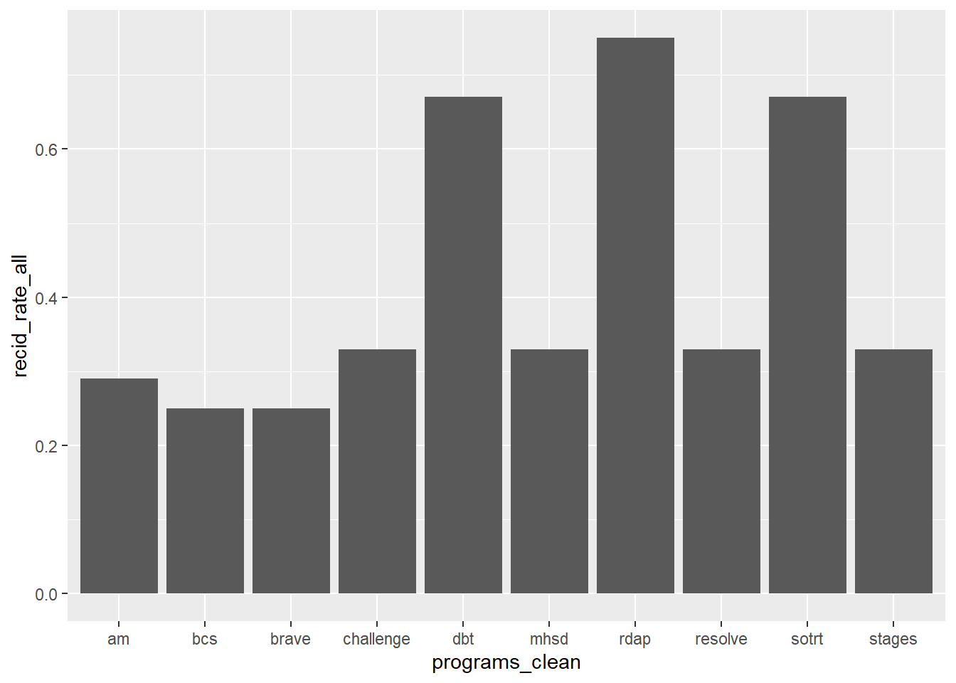
#basic bar chart of recidivism rate by year by program
ggplot(tabout,aes(x=programs_clean, y=recid_rate_year,fill=year)) +
         geom_bar(position="dodge", stat="identity")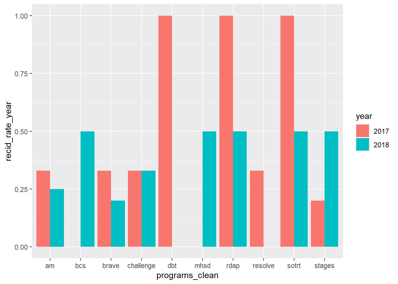
Oh I think we could do better than that!
#build bar chart of recidivism rates across programs
#information to plot, pick dates
dates <- as.numeric(c(date1,date2)) #what years of data do you want to plot?

#custom title header of plot
titledates <- ifelse(length(dates)>=2 & date1 != date2, paste0(date1," - ",date2),
                     ifelse((dates==date1 | dates==date2) & ALL.BY, as.character(dates),
                            ifelse(!ALL.BY, date1, "")))

#which years/programs are missing data?
prg.NA <- tabout |>
  filter(is.na(recid_rate_year)) |>
  pull(programs_clean)

#caption text about missing program data
{if(length(prg.NA)!=0) cond.text <- capture.output(cat("The following programs were missing data in some years:", unique(toupper(prg.NA)), sep=" ")) else cond.text <- ""}

#plot it! this will plot recidivism rates with overlaid staffing text
rr <- ggplot(tabout |>
               filter(if(ALL.BY) year %in% dates else year == date2) |>
               mutate(recid_rate = case_when(ALL.BY  ~ recid_rate_year,
                                             !ALL.BY ~ recid_rate_all))
             ,aes(x=programs_clean, y=recid_rate, fill=year)) +
  geom_bar(position = "dodge",stat = "identity", na.rm=TRUE) +
  geom_text(aes(label=ifelse(year==dates[2],paste(num_staff,"staff"),"")), vjust=-0.3, color = staffc, na.rm=TRUE) +
  scale_fill_manual(values=c(date1c,date2c)) +
  ylim(0,1) +
  ylab("Recidivism Rate") +
  xlab("EBRR Programs") +
  ggtitle(paste0("Recidivism Rates across EBRR programs\n",titledates)) +
  theme_classic() +
  #remove legend if plotting overall (not by year)
  {if(!ALL.BY) theme(legend.position="none")}+
  #only print caption if a program is missing data
  labs(caption = cond.text) +
  theme(plot.caption=element_text(hjust=0))

#display
rr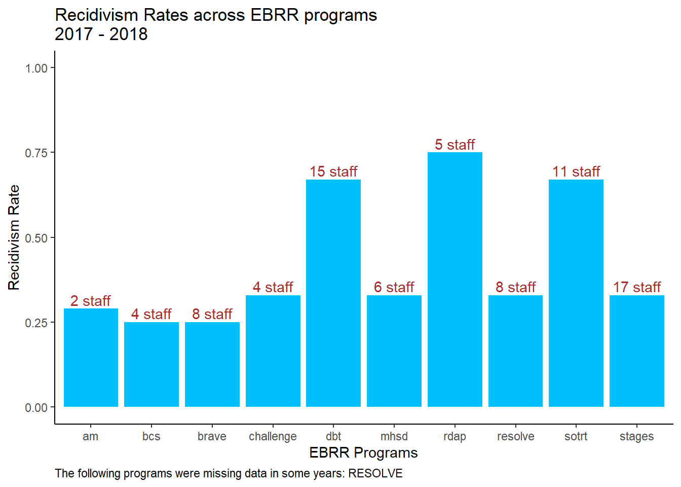
#keep or hide legend depending on overall or by years
{if (ALL.BY) cond.leg <- T else cond.leg <- F}

hc_setup <- highchart() |>
  hc_tooltip(formatter = JS("function(){return(this.point.tooltip)}")) |>
  hc_title(text = paste0("Recidivism Rates across EBRR programs\n",titledates)) |>
  hc_xAxis(title = list(text = "EBRR Programs"), type = "category", labels = list(style = list(width = 200))) |>
  hc_yAxis(title = list(text = "Recidivism Rate"), max = 1) |>
  hc_legend(enabled = cond.leg) |>
  hc_caption(text = cond.text) |>
  hc_add_dependency(name = "modules/exporting.js") |>
  hc_exporting(enabled = TRUE,
               chartOptions  = list(
                 chart = list(
                   backgroundColor = 'white')),
               buttons       = list(
                 contextButton = list(
                   menuItems = list("downloadPNG", "downloadSVG"))))
#overall
{if (!ALL.BY)
hc_setup |>
  hc_add_series(data = tabout |>
                  filter(year == date2) |>
                  mutate(tooltip = paste0("<b>", program_official, "</b><br>",
                                   "Recidivism Rate: ",recid_rate_all, "<br>",
                                   "Staffing: ", num_staff)),
                hcaes(x=program_official, y=recid_rate_all),
                color = "lightblue",
                type  = "bar")
}

#by year
{if (ALL.BY)
hc_setup |>
  hc_add_series(data = tabout |>
                  filter(year %in% dates) |>
                  mutate(tooltip = paste0("<b>", program_official, "</b><br>",
                                   "Recidivism Rate: ",recid_rate_year, "<br>",
                                   "Staffing: ", num_staff)),
                hcaes(x=program_official, y=recid_rate_year, group=year),
                color = c("lightblue","darkgreen"),
                type  = "bar")
}Save this for the final report!
This was amazing work; our Director is so happy! But wait! Oh no!! The Center Wing Coalition advocacy group just published a report that EBRR programs’ recidivism rates are at an all time high of 47.4% with a report that claims to have used your DOC’s reported data on EBRR program recidivism rates! Find out what’s going on, and fast!
#manage the data to produce recidivism rates
tabout2 <- inner_join(roster2, staff2, by = ("programs_clean")) |>
  ungroup() |>
  #if any years are missing, fill in
  complete(year, nesting(programs_clean,num_staff),
           fill = list(recid_rate_all = NA, recid_rate_year = NA)
  ) |>
  #correct missing values for recid_rate_all since this is the overall recidivism rate across multiple years
  group_by(programs_clean) |>
  fill(c(recid_rate_all,clients_served_all), .direction = "updown")

#calculate average recidivism rate across programs from all years
unw.a <- round(mean(tabout2$recid_rate_all,na.rm=TRUE),2)

#calculate average recidivism rate across programs from year 1
unw.d1 <- round(mean(tabout2[which(tabout2$year==date1),]$recid_rate_year,na.rm=TRUE),2)

#calculate average recidivism rate across programs from year 2
unw.d2 <- round(mean(tabout2[which(tabout2$year==date2),]$recid_rate_year,na.rm=TRUE),2)

#JUST 5 PROGRAMS!
#calculate average recidivism rate across programs from all years
unw.a5 <- round(mean(tabout2[which(!tabout2$programs_clean %in% rm.pgms),]$recid_rate_all,na.rm=TRUE),2)

#calculate average recidivism rate across programs from year 1
unw.d15 <- round(mean(tabout2[which(tabout2$year==date1 & !tabout2$programs_clean %in% rm.pgms),]$recid_rate_year,na.rm=TRUE),2)

#calculate average recidivism rate across programs from year 2
unw.d25 <- round(mean(tabout2[which(tabout2$year==date2 & !tabout2$programs_clean %in% rm.pgms),]$recid_rate_year,na.rm=TRUE),2)


#verify join was successful
doublecheck <- anti_join(roster2, staff2, by = ("programs_clean"))

#print values
print(paste0(unw.a*100,"%", " average recidivism rate overall"))
print(paste0(unw.d1*100,"%", " average recidivism rate in ",date1))
print(paste0(unw.d2*100,"%", " average recidivism rate in ",date2))
[1] "42% average recidivism rate overall"
[1] "45% average recidivism rate in 2017"
[1] "36% average recidivism rate in 2018"Hm - something still doesn’t line up. We need to keep investigating and find out why our numbers aren’t matching up!
#programs to remove per the CWC report
rm.pgms <- c("bcs", "brave", "sotrt", "mhsd", "resolve")#remove 5 of the 10 programs because the advocacy group was sneaky
adv <- tabout |>
filter(!(programs_clean %in% rm.pgms) &
year == date1) #dates repeat the same information, so just pick one date to average over
#calculate ADVOCACY rate, which will be inserted into document text
adv_rate <- round(mean(adv$recid_rate_all,na.rm=TRUE)*100,1)
cat(capture.output(cat(paste0(adv_rate,"%"), "average recidivism rate overall for the following programs:", unique(tabout[which(!tabout$programs_clean %in% rm.pgms),]$programs_clean), sep=" ")))47.4% average recidivism rate overall for the following programs: am challenge dbt rdap stagesAlright - there’s the number the advocacy group reported. But what’s missing? Our Director is not going to be satisfied with just replicating the Center Wing Coalition results! What if we considered calculating a weighted recidivism rate?
#manage the data to produce recidivism rates
#total clients served (all years, year1, year2)
total.a <- sum(tabout2[which(tabout2$year==date1),]$clients_served_all, na.rm=TRUE)
tabout2.wgt <- tabout2 |>
  filter(year==date1) |>
  mutate(recid_rate_all_w = clients_served_all*recid_rate_all)
w.a <- round(sum(tabout2.wgt$recid_rate_all_w)/total.a,2)

#total clients served (year 1)
total.d1 <- sum(tabout2[which(tabout2$year==date1),]$clients_served_year,na.rm=TRUE)
tabout2.wgt <- tabout2 |>
  filter(year==date1) |>
  mutate(recid_rate_year_w = clients_served_year*recid_rate_year)
w.d1 <- round(sum(tabout2.wgt$recid_rate_year_w,na.rm=TRUE)/total.d1,2)

#total clients served (year2)
total.d2 <- sum(tabout2[which(tabout2$year==date2),]$clients_served_year,na.rm=TRUE)
tabout2.wgt <- tabout2 |>
  filter(year==date2) |>
  mutate(recid_rate_year_w = clients_served_year*recid_rate_year)
w.d2 <- round(sum(tabout2.wgt$recid_rate_year_w,na.rm=TRUE)/total.d2,2)

#JUST 5 PROGRAMS!!!
#total clients served (all years)
total.a5 <- sum(tabout2[which(tabout2$year==date1 & !tabout2$programs_clean %in% rm.pgms),]$clients_served_all, na.rm=TRUE)
tabout2.wgt5 <- tabout2 |>
  filter(!(programs_clean %in% rm.pgms) & year==date1) |>
  mutate(recid_rate_all_w = clients_served_all*recid_rate_all)
w.a5 <- round(sum(tabout2.wgt5$recid_rate_all_w)/total.a5,2)

#total clients served (year 1)
total.d15 <- sum(tabout2[which(tabout2$year==date1 & !tabout2$programs_clean %in% rm.pgms),]$clients_served_year,na.rm=TRUE)
tabout2.wgt5 <- tabout2 |>
  filter(!(programs_clean %in% rm.pgms) & year==date1) |>
  mutate(recid_rate_year_w = clients_served_year*recid_rate_year)
w.d15 <- round(sum(tabout2.wgt5$recid_rate_year_w,na.rm=TRUE)/total.d15,2)

#total clients served (year2)
total.d25 <- sum(tabout2[which(tabout2$year==date2 & !tabout2$programs_clean %in% rm.pgms),]$clients_served_year,na.rm=TRUE)
tabout2.wgt5 <- tabout2 |>
  filter(!(programs_clean %in% rm.pgms) & year==date2) |>
  mutate(recid_rate_year_w = clients_served_year*recid_rate_year)
w.d25 <- round(sum(tabout2.wgt5$recid_rate_year_w,na.rm=TRUE)/total.d25,2)


#print values
print(paste0(w.a*100,"%", " average recidivism rate (weighted) overall"))
print(capture.output(cat(paste0(w.a5*100,"%"), "average recidivism rate (weighted) overall for the following programs:", unique(tabout[which(!tabout$programs_clean %in% rm.pgms),]$programs_clean), sep=" ")))
[1] "38% average recidivism rate (weighted) overall"
[1] "41% average recidivism rate (weighted) overall for the following programs: am challenge dbt rdap stages"Alright! If we just weight our data then we see that the average overall recidivism rate across the five programs that the advocacy group highlighted is only 41%. Great work!
Now let’s report it through some fancy data visualization work.
Change the highlighted code below (ALL.BY, CWC, and plot colors) to update your output.
A Download Image button will appear when you hover over the plot.
Let’s prepare our data to do some really fun data viz! What are some other engaging ways we could plot recidivism rates for leadership and our stakeholders pooled overall for these programs?
#this code will run if plotting data for multiple years, otherwise nothing will be produced (i.e., ALL.BY <- T)

#manipulate data for plotting
tabout.date1 <- tabout |>
  filter(year==date1) |>
  select(c(recid_rate_year, programs_clean, recid_rate_all)) |>
  rename(recid_rate_date1 = recid_rate_year)
tabout.date2 <- tabout |>
  filter(year==date2) |>
  select(c(recid_rate_year, programs_clean)) |>
  rename(recid_rate_date2 = recid_rate_year)
tabout.dates <- inner_join(tabout.date1, tabout.date2, by = "programs_clean") |>
  select(programs_clean, recid_rate_date1, recid_rate_date2, recid_rate_all)

#make some really cool horizontal floating dot charts!
#overwrite value of rates to overall if ALL.BY
{if(!ALL.BY) tabout.dates$recid_rate_date1 <- tabout.dates$recid_rate_all}

#plot two years or one year depending on ALL.BY setting
{if(ALL.BY) plotit <- c(tabout.dates[which(tabout.dates$programs_clean=="stages"),]$recid_rate_date1, tabout.dates[which(tabout.dates$programs_clean=="stages"),]$recid_rate_date2) else plotit <- tabout.dates[which(tabout.dates$programs_clean=="stages"),]$recid_rate_date1}

#remove label legend if by year
{if(ALL.BY) titledates2 <- c(as.factor(date1),as.factor(date2)) else titledates2 <- ""}

#plot!
gg_dot <- tabout.dates |>
  # rearrange the factor levels for programs by rates for date1
  arrange(recid_rate_date1) |>
  mutate(discipline = fct_inorder(programs_clean)) |>

  ggplot() +
  # remove axes and superfluous grids
  theme_classic() +
  theme(axis.title = element_blank(),
        axis.ticks.y = element_blank(),
        axis.line = element_blank()) +

  # add a dummy point for scaling purposes
  geom_point(aes(x = 0.7, y = programs_clean),
             size = 0, col = "white") +

  # add the horizontal programs_clean lines
  geom_hline(yintercept = 1:length(tabout.dates$programs_clean), col = "grey80") +

  # add a point for each date1 recidivism rate
  geom_point(aes(x = recid_rate_date1, y = programs_clean),
             size = 11, col = date1c) +

  # add a point for each date2 recidivism rate
 {if(ALL.BY) geom_point(aes(x = recid_rate_date2, y = programs_clean),size = 11, col = date2c)} +

  # round each date2 recidivism rate
  {if(ALL.BY) geom_text(aes(x = recid_rate_date2, y = programs_clean, label = paste0(round(recid_rate_date2, 2))), col = "black")} +

  # round each date1 recidivism rate
  geom_text(aes(x = recid_rate_date1, y = programs_clean,
                label = paste0(round(recid_rate_date1, 2))),
            col = "white") +

  # add a label above the first two points
  geom_text_repel(aes(x = x, y = y, label = label, col = label), force_pull = 50,
            data.frame(x     = plotit,
                       y     = length(tabout.dates$programs_clean) + 2,
                       label = titledates2), size = 6) +
  scale_color_manual(values = c(date1c, date2c), guide = "none") +

  # manually specify the x-axis
  scale_x_continuous(breaks = c(0, 0.25, 0.5, 0.75, 1),
                     labels = c("0","0.25", "0.50", "0.75", "1")) +
  # manually set the spacing above and below the plot
  scale_y_discrete(expand = c(0.2, 0))

#add titles/captions
gg_dot +
  {if (ALL.BY) ggtitle("Recidivism Rates across EBRR programs\n") else ggtitle(paste0("Recidivism Rates across EBRR programs\n",titledates))} +
  #only print caption if a program is missing data
  labs(caption = cond.text) +
  theme(plot.caption=element_text(hjust=0))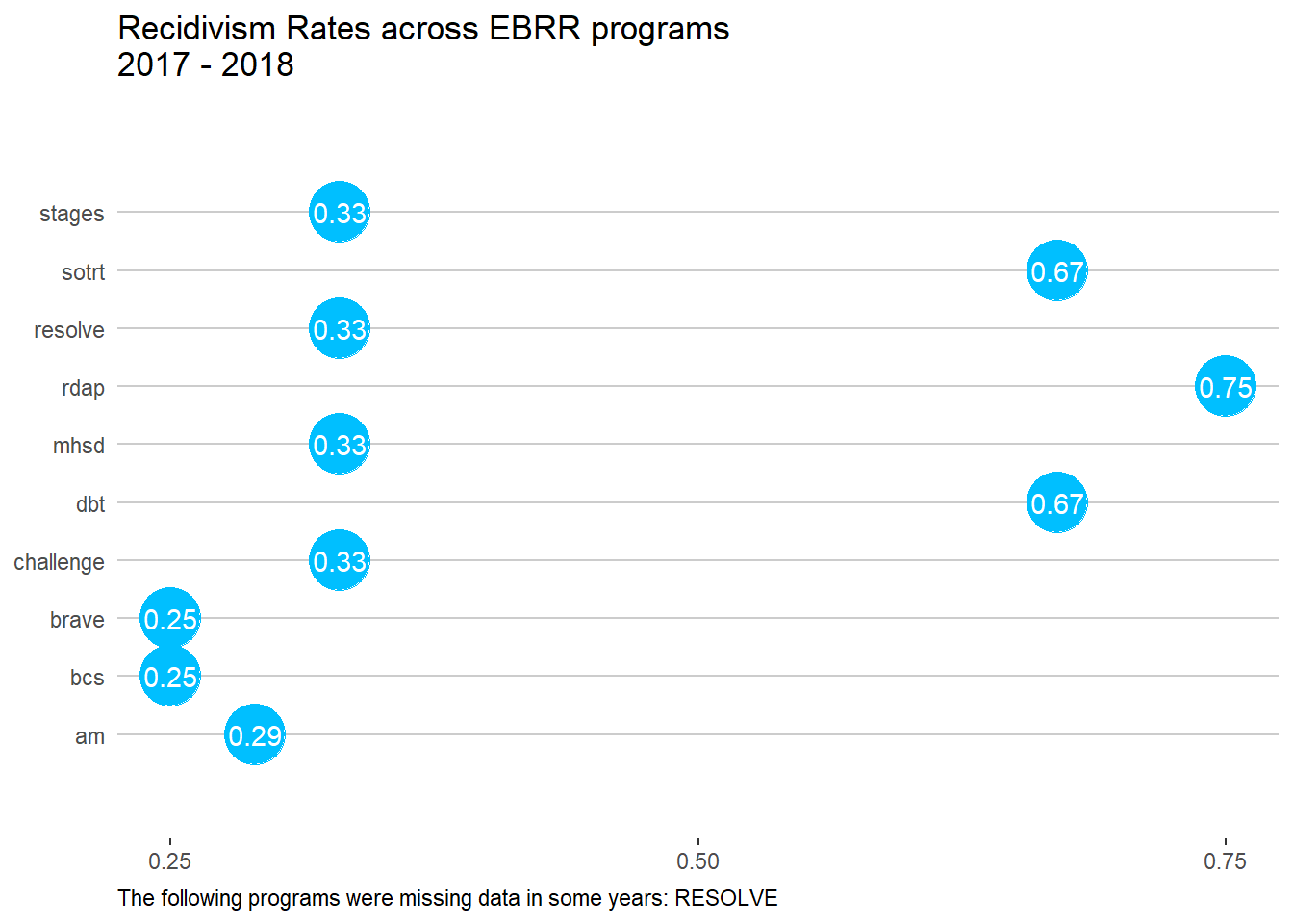
##horizontal lollipop chart
ggplot(tabout, aes(x=programs_clean, y=recid_rate_all)) +
  geom_segment( aes(x=programs_clean, xend=programs_clean, y=0, yend=recid_rate_all), color=date1c) +
  geom_point( color=staffc, size=4, alpha=0.6) +
  theme_light() +
  coord_flip() +
  xlab("EBRR Programs") +
  ylab("Recidivism Rate") +
  theme(
    panel.grid.major.y = element_blank(),
    panel.border = element_blank(),
    axis.ticks.y = element_blank()
  ) +
  ggtitle(paste0("Recidivism Rates across EBRR programs\n",titledates)) +
  theme(plot.caption=element_text(hjust=0)) +
  #only print caption if a program is missing data
  labs(caption = cond.text)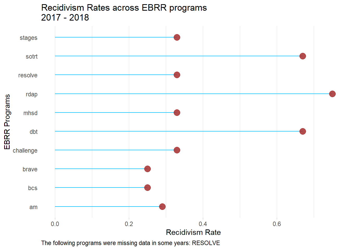
##horizontal lollipop chart w/weighted average
ggplot(tabout, aes(x=programs_clean, y=recid_rate_all)) +
  geom_segment(aes(x=programs_clean, xend=programs_clean, y=w.a, yend=recid_rate_all), color=date1c) +
  geom_point(color=staffc, size=4, alpha=0.6) +
  geom_hline(yintercept=w.a, linetype = "dashed", color = hlinew1, size = 1) +
  geom_label(aes(label=paste0("Weighted avg: ",w.a), x=w.a, vjust = -9, hjust = 0.75), fill=hlinew1,
                  data = tabout |>
               filter(programs_clean == last & year == date2)) +
  theme_light() +
  coord_flip() +
  xlab("EBRR Programs") +
  ylab("Recidivism Rate") +
  theme(
    panel.grid.major.y = element_blank(),
    panel.border = element_blank(),
    axis.ticks.y = element_blank()
  ) +
  ggtitle(paste0("Recidivism Rates across EBRR programs\n",titledates)) +
  #only print caption if a program is missing data
  labs(caption = cond.text) +
  theme(plot.caption=element_text(hjust=0))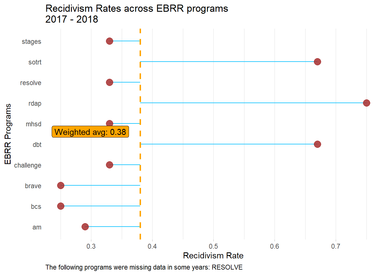
What about displaying these rates by release year?
#this code will run if plotting data for multiple years, otherwise nothing will be produced (i.e., ALL.BY <- T)

#manipulate data for plotting
tabout.date1 <- tabout |>
  filter(year==date1) |>
  select(c(recid_rate_year, programs_clean, recid_rate_all)) |>
  rename(recid_rate_date1 = recid_rate_year)
tabout.date2 <- tabout |>
  filter(year==date2) |>
  select(c(recid_rate_year, programs_clean)) |>
  rename(recid_rate_date2 = recid_rate_year)
tabout.dates <- inner_join(tabout.date1, tabout.date2, by = "programs_clean") |>
  select(programs_clean, recid_rate_date1, recid_rate_date2, recid_rate_all)

#make some really cool horizontal floating dot charts!
#overwrite value of rates to overall if ALL.BY
{if(!ALL.BY) tabout.dates$recid_rate_date1 <- tabout.dates$recid_rate_all}

#plot two years or one year depending on ALL.BY setting
{if(ALL.BY) plotit <- c(tabout.dates[which(tabout.dates$programs_clean=="stages"),]$recid_rate_date1, tabout.dates[which(tabout.dates$programs_clean=="stages"),]$recid_rate_date2) else plotit <- tabout.dates[which(tabout.dates$programs_clean=="stages"),]$recid_rate_date1}

#remove label legend if by year
{if(ALL.BY) titledates2 <- c(as.factor(date1),as.factor(date2)) else titledates2 <- ""}

#plot!
gg_dot <- tabout.dates |>
  # rearrange the factor levels for programs by rates for date1
  arrange(recid_rate_date1) |>
  mutate(discipline = fct_inorder(programs_clean)) |>

  ggplot() +
  # remove axes and superfluous grids
  theme_classic() +
  theme(axis.title = element_blank(),
        axis.ticks.y = element_blank(),
        axis.line = element_blank()) +

  # add a dummy point for scaling purposes
  geom_point(aes(x = 0.7, y = programs_clean),
             size = 0, col = "white") +

  # add the horizontal programs_clean lines
  geom_hline(yintercept = 1:length(tabout.dates$programs_clean), col = "grey80") +

  # add a point for each date1 recidivism rate
  geom_point(aes(x = recid_rate_date1, y = programs_clean),
             size = 11, col = date1c) +

  # add a point for each date2 recidivism rate
 {if(ALL.BY) geom_point(aes(x = recid_rate_date2, y = programs_clean),size = 11, col = date2c)} +

  # round each date2 recidivism rate
  {if(ALL.BY) geom_text(aes(x = recid_rate_date2, y = programs_clean, label = paste0(round(recid_rate_date2, 2))), col = "black")} +

  # round each date1 recidivism rate
  geom_text(aes(x = recid_rate_date1, y = programs_clean,
                label = paste0(round(recid_rate_date1, 2))),
            col = "white") +

  # add a label above the first two points
  geom_text_repel(aes(x = x, y = y, label = label, col = label), force_pull = 50,
            data.frame(x     = plotit,
                       y     = length(tabout.dates$programs_clean) + 2,
                       label = titledates2), size = 6) +
  scale_color_manual(values = c(date1c, date2c), guide = "none") +

  # manually specify the x-axis
  scale_x_continuous(breaks = c(0, 0.25, 0.5, 0.75, 1),
                     labels = c("0","0.25", "0.50", "0.75", "1")) +
  # manually set the spacing above and below the plot
  scale_y_discrete(expand = c(0.2, 0))

#add titles/captions
gg_dot +
  {if (ALL.BY) ggtitle("Recidivism Rates across EBRR programs\n") else ggtitle(paste0("Recidivism Rates across EBRR programs\n",titledates))} +
  #only print caption if a program is missing data
  labs(caption = cond.text) +
  theme(plot.caption=element_text(hjust=0))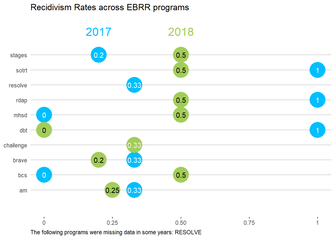
#plot!
gg_line <- tabout.dates |>
  # add a variable for when rates are higher in date1 than in date2 (for colours)
  mutate(date1high = recid_rate_date1 > recid_rate_date2) |>
  ggplot() +
  # add a line segment that goes from date1 to date2 for each program
  geom_segment(aes(x     = 1,                xend = 2,
                   y     = recid_rate_date1, yend = recid_rate_date2,
                   group = programs_clean,
                   col = date1high),
               size = 1.2) +
  # set the colors
  scale_color_manual(values = c(date1c, date2c), guide = "none")  +
  # remove all axis stuff
  theme_classic() +
  theme(axis.line  = element_blank(),
        axis.text  = element_blank(),
        axis.title = element_blank(),
        axis.ticks = element_blank()) +
  # add vertical lines that act as axis for date1
  geom_segment(x    = 1,
               xend = 1,
               y    = min(tabout.dates$recid_rate_date1, na.rm=T) - 0.1,
               yend = max(tabout.dates$recid_rate_date1, na.rm=T) + 0.125,
               col  = "grey70", size = 0.5) +
  # add vertical lines that act as axis for date2
  geom_segment(x    = 2,
               xend = 2,
               y    = min(tabout.dates$recid_rate_date1, na.rm=T) - 0.1,
               yend = max(tabout.dates$recid_rate_date1, na.rm=T) + 0.125,
               col  = "grey70", size = 0.5) +
  # add the labels above their axes
  geom_text(aes(x = x, y = y, label = label),
            data = data.frame(x = 1:2,
                              y = max(tabout.dates$recid_rate_date2, na.rm=T) + 0.05,
                              label = c(date1, date2)),
            col = "grey30",
            size = 6)  +
  # add the label and rate for each program next the date1 axis
  geom_text_repel(aes(x     = 1 - 0.03,
                      y     = recid_rate_date1,
                      label = paste0(programs_clean, ", ", round(recid_rate_date1, 2))),
             force_pull   = 0,
             nudge_y      = 0.05, nudge_x = -0.075,
             direction    = "y",
             hjust        = 1,
             segment.size = 0.2,
             max.iter = 1e4, max.time = 1) +
  # add the rate next to each point on the date2 axis
  geom_text(aes(x = 2 + 0.08,
                y = recid_rate_date2,
                label = paste0(round(recid_rate_date2, 2))),
            col = "grey30") +
  # set the limits of the x-axis so that the labels are not cut off
  scale_x_continuous(limits = c(0.5, 2.1)) +

  # add the white outline for the points at each rate for date1
  geom_point(aes(x = 1,
                 y = recid_rate_date1), size = 4.5,
             col = "white") +
  # add the white outline for the points at each rate for date2
  geom_point(aes(x = 2,
                 y = recid_rate_date2), size = 4.5,
             col = "white") +

  # add the actual points at each rate for date1
  geom_point(aes(x = 1,
                 y = recid_rate_date1), size = 4,
             col = "grey60") +
  # add the actual points at each rate for date2
  geom_point(aes(x = 2,
                 y = recid_rate_date2), size = 4,
             col = "grey60")

gg_line +
  ggtitle("Recidivism Rates across EBRR programs\n") +
  #only print caption if a program is missing data
  labs(caption = cond.text) +
  theme(plot.caption=element_text(hjust=0))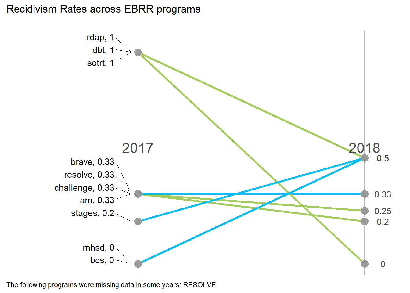
highchart() |>
  hc_add_series(data = tabout |>
                  filter(year %in% dates) |>
                  mutate(recid_rate = ifelse(year == date1, -1*recid_rate_year, recid_rate_year),
                         tooltip    = paste0("<b>", program_official, "</b><br>",
                                             "Recidivism Rate: ", abs(recid_rate), "<br>",
                                             "Staffing: ", num_staff)),
                hcaes(x=program_official, y=recid_rate, group=year),
                color = c("lightblue","darkgreen"),
                type  = "bar",
                showInLegend = F) |>
  hc_plotOptions(bar = list(stacking = "normal")) |>
  # format the labels on the x-axis (y-axis per HC)
  hc_yAxis(labels = list(formatter = htmlwidgets::JS(
           "function() {return Math.abs(this.value); /* all labels to absolute values */
            }"
           )), title = list(text = "Recidivism Rate"), min = -1, max = 1) |>
  hc_tooltip(formatter = JS("function(){return(this.point.tooltip)}")) |>
  hc_xAxis(title = list(text = "EBRR Programs"), type = "category", labels = list(style = list(width = 200))) |>
  hc_caption(text = cond.text) |>
  hc_title(   text = date1, align = "center", x = 0, y = 20, margin = 0,
              style = list(fontSize = "12px", color = "lightblue")) |>
  hc_subtitle(text = date2, align = "center", x = 250, y = 20, margin = 0,
style = list(fontSize = "12px", color = "darkgreen"))This exploratory document has been really useful for our internal purposes! But what if we want to get all of the pertinent info into a single report for your Director in a format they can actually digest; something similar to the original report?
 [1] ---
 [2] title: "GDOC Program Recidivism/Staffing Requirements"
 [3] subtitle: "`r format(Sys.Date(), '%B %Y')`"
 [4] geometry: "left=1.5cm,right=1.5cm,top=0cm,bottom=1cm"
 [5] ---
 [6] \\setlength{\\headsep}{-0.25cm}
 [7] \\pagenumbering{gobble}
 [8] \\vspace{-2.6truecm}
 [9] ```{r pretable, echo=FALSE, message=FALSE, warning=FALSE}
[10] library(charlatan)
[11] library(lubridate)
[12] library(tidyverse)
[13] library(knitr)
[14] library(ggrepel)
[15] #data setup
[16] source("data_setup.R")
[17] source("re_report.R")
[18] source("execute.R")
[19] source("toggle.R")
[20] ```
[21] This report includes the overall recidivism rates (release years `r date1`-`r date2`) for evidence-based programming provided in the Gotham Department of Corrections facilities for high-risk people. Staffing numbers describe how many full-time employees are needed over the course of a year to keep each program running. Each program facilitator completes extensive training and must complete eight hours of continuing education each year.
[22] \\small
[23] ```{r table, echo=FALSE, message=FALSE, warning=FALSE}
[24] #programs to remove per the CWC report
[25] source("rm_pgms.R")
[26] #deduplicate across all columns
[27] source("dedup.R")
[28] #clean program names
[29] source("roster_clean.R")
[30] ##create dataset of numerators and denominators
[31] #recidivism rates overall
[32] source("rates.R")
[33] #clean program names
[34] source("staff_clean.R")
[35] #create table dataset
[36] source("tabledata.R")
[37] source("finaltable_report.R")
[38] reportit |> rename(`Program (Graduated 2017-2018)`          = "program_official",
[39]                    `Recidivism Rate (2018-2019)` = "recid_rate_all",
[40]                    Staffing          = "num_staff") |>
[41]   kable()
[42] ```
[43] \\vspace{-0.5truecm}
[44] ```{r graphic, include=FALSE}
[45] source2 <- function(file, start, end, ...) {
[46]     file.lines <- scan(file, what=character(), skip=start-1, nlines=end-start+1, sep='\\n')
[47]     file.lines.collapsed <- paste(file.lines, collapse='\\n')
[48]     source(textConnection(file.lines.collapsed), ...)
[49] }
[50] #manage the data to produce recidivism rates
[51] source("cwc_unw.R")
[52] #manage the data to produce recidivism rates
[53] #total clients served (all years, year1, year2)
[54] source("cwc_w.R")
[55] #build bar chart of recidivism rates across programs
[56] source2("va_cs_webr.qmd",42,133)
[57] #plot print
[58] pdf(width=6.5,height=5,pointsize=15,file="rrfinal.pdf")
[59] print(rrfinal)
[60] dev.off()
[61] ggsave("rrfinal.png", width = 8, height = 6, units = "in")
[62] ```
[63] \\begin{figure}
[64] \\includegraphics{rrfinal.pdf}
[65] \\end{figure}
[66] \\normalsize
[67] \\vspace{-1truecm}
[68] ## Findings
[69] \\vspace{-0.4cm}
[70] Overall, the program with the lowest recidivism rates is: `r reportit[which(reportit$recid_rate_all == min(reportit$recid_rate_all)),]$program_official`. The program with the highest recidivism rates is: `r reportit[which(reportit$recid_rate_all == max(reportit$recid_rate_all)),]$program_official`. The average weighted recidivism rate is `r w.a`.
[71] \\vspace{-0.3cm}
[72] ## Methodology
[73] \\vspace{-0.4cm}
[74] All participants have taken one of these programs right before release. The cohort analyzed were released from prison in `r date1` and `r date2`. Overall recidivism rates are computed. #for reproducibility
si <- sessioninfo::session_info()
si$packages$library <- NULL
si$platform$pandoc <- NULL
si
## ─ Session info ───────────────────────────────────────────────────────────────
## setting value
## version R version 4.4.1 (2024-06-14 ucrt)
## os Windows 10 x64 (build 19045)
## system x86_64, mingw32
## ui RTerm
## language (EN)
## collate English_United States.utf8
## ctype English_United States.utf8
## tz America/Chicago
## date 2024-08-15
##
## ─ Packages ───────────────────────────────────────────────────────────────────
## ! package * version date (UTC) lib source
## P askpass 1.2.0 2023-09-03 [] CRAN (R 4.4.1)
## P assertthat 0.2.1 2019-03-21 [] CRAN (R 4.4.1)
## P b64 0.1.1 2024-07-01 [] CRAN (R 4.4.1)
## P backports 1.5.0 2024-05-23 [] CRAN (R 4.4.0)
## P base64enc 0.1-3 2015-07-28 [] CRAN (R 4.4.0)
## P broom 1.0.6 2024-05-17 [] CRAN (R 4.4.1)
## P bslib 0.7.0 2024-03-29 [] CRAN (R 4.4.1)
## P bsplus 0.1.4 2022-11-16 [] CRAN (R 4.4.1)
## P cachem 1.1.0 2024-05-16 [] CRAN (R 4.4.1)
## P charlatan * 0.5.1 2023-09-13 [] CRAN (R 4.4.1)
## P checkmate 2.3.2 2024-07-29 [] CRAN (R 4.4.1)
## P cli 3.6.3 2024-06-21 [] CRAN (R 4.4.1)
## P codetools 0.2-20 2024-03-31 [] CRAN (R 4.4.1)
## P colorspace 2.1-0 2023-01-23 [] CRAN (R 4.4.1)
## P crosstalk * 1.2.1.9000 2024-08-01 [] Github (rstudio/crosstalk@4f76bd6)
## P curl 5.2.1 2024-03-01 [] CRAN (R 4.4.1)
## P data.table 1.15.4 2024-03-30 [] CRAN (R 4.4.1)
## P devtools * 2.4.5 2022-10-11 [] CRAN (R 4.4.1)
## P digest 0.6.36 2024-06-23 [] CRAN (R 4.4.1)
## P downloadthis * 0.4.0 2024-07-04 [] CRAN (R 4.4.1)
## P dplyr * 1.1.4 2023-11-17 [] CRAN (R 4.4.1)
## P DT * 0.33 2024-04-04 [] CRAN (R 4.4.1)
## P ellipsis 0.3.2 2021-04-29 [] CRAN (R 4.4.1)
## P evaluate 0.24.0 2024-06-10 [] CRAN (R 4.4.1)
## P fansi 1.0.6 2023-12-08 [] CRAN (R 4.4.1)
## P farver 2.1.2 2024-05-13 [] CRAN (R 4.4.1)
## P fastmap 1.2.0 2024-05-15 [] CRAN (R 4.4.1)
## P forcats * 1.0.0 2023-01-29 [] CRAN (R 4.4.1)
## P fs 1.6.4 2024-04-25 [] CRAN (R 4.4.1)
## P generics 0.1.3 2022-07-05 [] CRAN (R 4.4.1)
## P ggplot2 * 3.5.1 2024-04-23 [] CRAN (R 4.4.1)
## P ggrepel * 0.9.5 2024-01-10 [] CRAN (R 4.4.1)
## P glue 1.7.0 2024-01-09 [] CRAN (R 4.4.1)
## P gtable 0.3.5 2024-04-22 [] CRAN (R 4.4.1)
## P highcharter * 0.9.4 2022-01-03 [] CRAN (R 4.4.1)
## P hms 1.1.3 2023-03-21 [] CRAN (R 4.4.1)
## P htmltools 0.5.8.1 2024-04-04 [] CRAN (R 4.4.1)
## P htmlwidgets 1.6.4 2023-12-06 [] CRAN (R 4.4.1)
## P httpuv 1.6.15 2024-03-26 [] CRAN (R 4.4.1)
## P igraph 2.0.3 2024-03-13 [] CRAN (R 4.4.1)
## P jquerylib 0.1.4 2021-04-26 [] CRAN (R 4.4.1)
## P jsonlite 1.8.8 2023-12-04 [] CRAN (R 4.4.1)
## P knitr * 1.48 2024-07-07 [] CRAN (R 4.4.1)
## P labeling 0.4.3 2023-08-29 [] CRAN (R 4.4.0)
## P later 1.3.2 2023-12-06 [] CRAN (R 4.4.1)
## P lattice 0.22-6 2024-03-20 [] CRAN (R 4.4.1)
## P lazyeval 0.2.2 2019-03-15 [] CRAN (R 4.4.1)
## P lifecycle 1.0.4 2023-11-07 [] CRAN (R 4.4.1)
## P lubridate * 1.9.3 2023-09-27 [] CRAN (R 4.4.1)
## P magick 2.8.4 2024-07-14 [] CRAN (R 4.4.1)
## P magrittr 2.0.3 2022-03-30 [] CRAN (R 4.4.1)
## P MASS 7.3-60.2 2024-04-26 [] CRAN (R 4.4.1)
## P matrixStats 1.3.0 2024-04-11 [] CRAN (R 4.4.1)
## P memoise 2.0.1 2021-11-26 [] CRAN (R 4.4.1)
## P mime 0.12 2021-09-28 [] CRAN (R 4.4.0)
## P miniUI 0.1.1.1 2018-05-18 [] CRAN (R 4.4.1)
## P munsell 0.5.1 2024-04-01 [] CRAN (R 4.4.1)
## P officer * 0.6.6 2024-05-05 [] CRAN (R 4.4.1)
## P openssl 2.2.0 2024-05-16 [] CRAN (R 4.4.1)
## P pander 0.6.5 2022-03-18 [] CRAN (R 4.4.1)
## P pillar 1.9.0 2023-03-22 [] CRAN (R 4.4.1)
## P pkgbuild 1.4.4 2024-03-17 [] CRAN (R 4.4.1)
## P pkgconfig 2.0.3 2019-09-22 [] CRAN (R 4.4.1)
## P pkgload 1.4.0 2024-06-28 [] CRAN (R 4.4.1)
## P plyr 1.8.9 2023-10-02 [] CRAN (R 4.4.1)
## P processx 3.8.4 2024-03-16 [] CRAN (R 4.4.1)
## P profvis 0.3.8 2023-05-02 [] CRAN (R 4.4.1)
## P promises 1.3.0 2024-04-05 [] CRAN (R 4.4.1)
## P pryr 0.1.6 2023-01-17 [] CRAN (R 4.4.1)
## P ps 1.7.7 2024-07-02 [] CRAN (R 4.4.1)
## P purrr * 1.0.2 2023-08-10 [] CRAN (R 4.4.1)
## P quantmod 0.4.26 2024-02-14 [] CRAN (R 4.4.1)
## P quarto * 1.4.4 2024-07-20 [] CRAN (R 4.4.1)
## P R6 2.5.1 2021-08-19 [] CRAN (R 4.4.1)
## P ragg 1.3.2 2024-05-15 [] CRAN (R 4.4.1)
## P rapportools 1.1 2022-03-22 [] CRAN (R 4.4.1)
## P Rcpp 1.0.13 2024-07-17 [] CRAN (R 4.4.1)
## P readr * 2.1.5 2024-01-10 [] CRAN (R 4.4.1)
## P remotes 2.5.0 2024-03-17 [] CRAN (R 4.4.1)
## renv 1.0.7 2024-04-11 [] CRAN (R 4.4.1)
## P reshape2 1.4.4 2020-04-09 [] CRAN (R 4.4.1)
## P rlang 1.1.4 2024-06-04 [] CRAN (R 4.4.1)
## P rlist 0.4.6.2 2021-09-03 [] CRAN (R 4.4.1)
## P rmarkdown * 2.27 2024-05-17 [] CRAN (R 4.4.1)
## P rstudioapi 0.16.0 2024-03-24 [] CRAN (R 4.4.1)
## P sass 0.4.9 2024-03-15 [] CRAN (R 4.4.1)
## P scales 1.3.0 2023-11-28 [] CRAN (R 4.4.1)
## P sessioninfo 1.2.2 2021-12-06 [] CRAN (R 4.4.1)
## P shiny 1.9.1 2024-08-01 [] CRAN (R 4.4.1)
## P stringi 1.8.4 2024-05-06 [] CRAN (R 4.4.0)
## P stringr * 1.5.1 2023-11-14 [] CRAN (R 4.4.1)
## P summarytools * 1.0.1 2022-05-20 [] CRAN (R 4.4.1)
## P summarywidget * 0.0.0.9000 2024-08-01 [] Github (kent37/summarywidget@c0da3f7)
## P systemfonts 1.1.0 2024-05-15 [] CRAN (R 4.4.1)
## P textshaping 0.4.0 2024-05-24 [] CRAN (R 4.4.1)
## P tibble * 3.2.1 2023-03-20 [] CRAN (R 4.4.1)
## P tidyr * 1.3.1 2024-01-24 [] CRAN (R 4.4.1)
## P tidyselect 1.2.1 2024-03-11 [] CRAN (R 4.4.1)
## P tidyverse * 2.0.0 2023-02-22 [] CRAN (R 4.4.1)
## P timechange 0.3.0 2024-01-18 [] CRAN (R 4.4.1)
## P TTR 0.24.4 2023-11-28 [] CRAN (R 4.4.1)
## P tzdb 0.4.0 2023-05-12 [] CRAN (R 4.4.1)
## P urlchecker 1.0.1 2021-11-30 [] CRAN (R 4.4.1)
## P usethis * 3.0.0 2024-07-29 [] CRAN (R 4.4.1)
## P utf8 1.2.4 2023-10-22 [] CRAN (R 4.4.1)
## P uuid 1.2-0 2024-01-14 [] CRAN (R 4.4.0)
## P vctrs 0.6.5 2023-12-01 [] CRAN (R 4.4.1)
## P whisker 0.4.1 2022-12-05 [] CRAN (R 4.4.1)
## P withr 3.0.0 2024-01-16 [] CRAN (R 4.4.1)
## P xfun 0.46 2024-07-18 [] CRAN (R 4.4.1)
## P xml2 1.3.6 2023-12-04 [] CRAN (R 4.4.1)
## P xtable 1.8-4 2019-04-21 [] CRAN (R 4.4.1)
## P xts 0.14.0 2024-06-05 [] CRAN (R 4.4.1)
## P yaml 2.3.9 2024-07-05 [] CRAN (R 4.4.1)
## P zip 2.3.1 2024-01-27 [] CRAN (R 4.4.1)
## P zoo 1.8-12 2023-04-13 [] CRAN (R 4.4.1)
##
##
## P ── Loaded and on-disk path mismatch.
##
## ──────────────────────────────────────────────────────────────────────────────